An initial evaluation of carbon proxies for dynamic reforestation baselines

SUMMARY

In this Research Brief, Pachama presents an initial demonstration of a dynamic baseline for reforestation projects. We tested four candidate proxies for tracking carbon gain in control areas, including optical and radar vegetation indices as well as canopy height, which Pachama estimates by combining satellite observations with training samples from airborne lidar. Both optical and radar vegetation indices presented significant limitations for computing accurate, reproducible dynamic baselines owing largely to their noisiness and weaker correlation with forest carbon. Most problematic were optical indices, which saturated early in reforestation (< 5 yrs), and subsequently became unusable for computing the baseline. Canopy height resolved each of these limitations, showing clear divergence between test sites and their control areas and remaining sensitive to heights expected in mature forest (~30m under Pachama v1 canopy height algorithm). Independent, “ground-truth” validation of carbon proxies remains essential to building public confidence in the accuracy and consistency of baselines across projects. We strongly urge coordinated effort among market stakeholders to build the policy and computational infrastructure required for such validation. 

INTRODUCTION

The rise of nature-based solutions as a component of corporate climate strategies has driven a large increase in investment in forest conservation and restoration projects within the voluntary carbon market. Transaction volume for forest carbon credits roughly doubled between 2020 and 2022, and currently represents nearly half of all credits transacted¹.

Yet, concerns persist about whether these projects are reducing emissions to the extent claimed. Core to a project’s claimed emissions impact is the concept of a baseline. The baseline is a project’s expected annual deforestation or reforestation, if it had not enrolled in the carbon market. The project’s emissions impact is, therefore, the difference between its realized carbon emissions and its baseline. An accurate, conservative baseline is critical to avoiding over-crediting (i.e., issuing a credit volume that exceeds the project’s actual emissions reductions or removals).

As Pachama has previously described, dynamic baselines offer a consistent, algorithmic approach to estimating background deforestation and reforestation rates in the absence of a carbon project. Under this approach, the baseline is simply the annually observed carbon change in a control area selected to match the project. Prior studies have used dynamic baselines to assess the integrity of issuance for avoided deforestation (primarily REDD+^a ) projects ^2–4. 

There is a growing need to demonstrate the approach for other project types, namely improved forest management (IFM) (e.g. Verra VM0045) and reforestation (ARR^b). This is particularly important, because, as we’ll also show here, the optimal data and methods for selecting control areas and quantifying their uncertainty remain an active area of research ^2–5.

Verra and the associated ABACUS label have recently required dynamic baselines for ARR projects (VM0047), a promising development for the carbon market.^c,d, Annual satellite-derived data of some measure of carbon change are necessary to quantify background carbon gain in the absence of an ARR project. VM0047 refers to this carbon proxy as a stocking index (SI). The ideal SI is obviously forest carbon itself, or a quantity highly correlated with forest carbon, such as canopy height. 

VM0047 specifies few SI requirements, effectively permitting a range of satellite-derived quantities, including vegetation indices derived from optical and radar observations (e.g. Normalized Difference Vegetation Index (NDVI), Enhanced Vegetation Index (EVI), Red Edge Index, Radar Normalized Difference Vegetation Index (RNDVI), Radar Vegetation Index (RVI), etc.) as well as two-dimensional forest attributes retrieved from satellite observations (e.g. canopy cover and leaf area index (LAI)). VM0047 simply requires the SI to be correlated with forest carbon, although the criteria for demonstrating sufficient correlation remain relatively undefined (Section 10.5 Data and Parameters Monitored, pp. 64-66) ¹².

In this Research Brief, we provide a demonstration of a dynamic ARR baseline for test sites in Pará, Brazil (Fig. 1).^e We discuss key data and methodological considerations, particularly the choice of a stocking index (SI), that are crucial to operationalizing dynamic ARR baselines for the market. We address the following questions that have important implications for a range of market stakeholders, including landowners, project developers, investors, and credit registries. 

1. What is the year of first issuance? When does the project’s SI time series diverge sufficiently from the control area, such that the project can issue its first credits? 
2. What is the year of SI saturation? When does the project’s SI stop increasing, despite continued forest growth in the project, rendering the SI unusable for computing the dynamic baseline? 
3. Does the SI produce accurate and consistent baselines? Can SI noise produce large variation in baseline estimates? Can SI noise produce large baselines, when the true baseline is near-zero? 
4. What is the minimum detectable baseline? What is the smallest possible baseline (i.e., carbon gain) the SI can reliably detect?

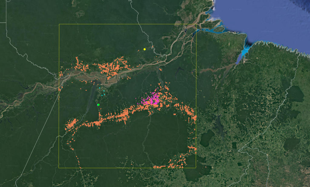
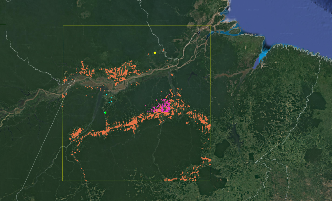
Fig. 1. Map of study area in Pará, Brazil.Study area (yellow box). Test forest regrowth sites (pasture to forest conversion in 2016) for demo implementation of dynamic control area baseline (n=2, green point). Constant Mapbiomas crop (cyan) and pasture (orange) cover 2000 – 2020 for quantifying stocking index (SI) stability over unchanging non-forest land cover. Pseudo-projects for quantifying uncertainty of control area selection. Pseudo-projects are defined as continuous Mapbiomas pasture 2000 – 2016 with unconstrained land use thereafter (n=30, magenta) (Fig. 8). Commercial plantation extracted from Du et al. (2022) to demonstrate dynamic baseline for test case of non-zero control area carbon gain (n=1, yellow point) (Fig. 9).

METHODS

 

Study area

Our study area in Pará, Brazil encompasses extensive intact forest, expanding pasture along the path of deforestation, and limited cropland (Fig. 1). The study area presents a simple environment for initial baseline tests, as we expect the true baseline to be near-zero. We expect a near-zero baseline, as Pachama canopy height maps (described below) showed insignificant net height gain (2015-2020) on areas classified as pasture and cropland. We used the Mapbiomas land cover product to identify land cover classes within the study area ^13,14. 

As we later discuss, a future priority will be evaluating SI performance in a more challenging environment with small but non-trivial background carbon gain. The urgent need is to characterize the minimum detectable baseline for SIs under a more rigorous treatment of SI uncertainty than the analysis presented here.

Test sites

We used annual Pachama canopy height datasets to manually delineate two test sites of sustained forest regrowth (height gain) within our study area. Both sites transitioned from pasture to forest in 2016 (Fig. 1). As the start year for Pachama’s initial canopy height product is 2015, we sought to identify test sites with reforestation shortly after 2015. We used Google Earth imagery to further visually confirm the year of non-forest-to-forest transition was 2016 (Fig. 2). For both test sites, which can be considered akin to passive reforestation ARR projects, we compute a dynamic baseline. 

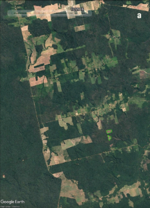
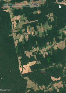
Fig. 2. Test forest regrowth sites. Pasture to forest conversion in 2016 for testing of dynamic control area baseline. a) Satellite imagery in December 2016 showing brown, non-forest cover showing and b) in December 2020 showing increased vegetation cover.

We initially used Mapbiomas land cover transitions to identify a larger potential set of test sites. 

However, due to uncertainty in the exact year of non-forest-to-forest transitions inherent to any land cover product, this larger pool of potential test sites requires more involved filtering beyond the scope of this Research Brief (e.g. break point analysis with longer SI time series).^f Hence, we share these two sites as an initial case study. 

Stocking indices (SI)

We computed a dynamic baseline for both test sites across four different candidate SIs: 

Landsat NDVI (Normalized Difference Vegetation Index) (30m resolution), higher resolution Sentinel-2 NDVI (10m), ALOS-Palsar radar RNDVI (Radar Normalized Difference Vegetation Index) (25m) , and a Pachama canopy height model (30m) derived from a suite of optical, radar, topographic, and climatological satellite observations (Fig. 3).

Landsat NDVI, Sentinel-2 NDVI, and ALOS-PALSAR RNDVI

We used Google Earth Engine (GEE) to acquire Landsat 8 Level 2, Collection 2, Tier 1 surface reflectance (LANDSAT/LC08/C02/T1_L2). We computed median annual image composites using the QA_PIXEL (cloud) and QA_RADSAT (radiometric saturations) bitwise masks to remove cloud-contaminated or otherwise saturated pixels. We used images from July – September due to the generally reduced cloud cover in these drier months. We then computed annual NDVI from the annual image composites.

Similarly, we acquired Sentinel-2 surface reflectance (COPERNICUS/S2_SR) and computed median annual image composites from July – September imagery. We used the QA60 (cloud and cirrus) bitwise masks to remove cloud-contaminated pixels prior to compositing and computed annual NDVI from the annual image composites. 

We acquired annual ortho-rectified, slope-corrected PALSAR radar imagery from the Global PALSAR-2/PALSAR Yearly Mosaic, version 2 collection (JAXA/ALOS/PALSAR/YEARLY/SAR_EPOCH). We computed annual RNDVI from these annual mosaics ¹⁵.

Pachama canopy height product

Pachama uses a multi-scale machine learning model to map canopy height. We produce regional maps of average top-of-canopy height using a combination of airborne lidar and a suite of satellite observations at varying spatial scales, including optical and radar imagery, topography, and climate data. We extract canopy height from airborne lidar as reference samples for model training. We train a variant of the boosted-tree machine learning model using the multi-scale satellite observations and the paired lidar-derived canopy height samples.

Our outputs include not only average canopy height for each spatial unit (i.e. a raster pixel) in the region, but also a measure of uncertainty for these predictions. Our mapping approach addresses two types of uncertainty: aleatoric (data uncertainty) and epistemic (model uncertainty) for canopy height estimates at both the pixel and regional level. In the coming months, Pachama expects to share a technical document summarizing our methods for canopy height mapping and an initial validation of map accuracy.

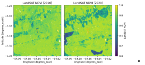
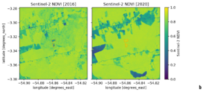
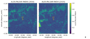
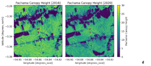
Fig. 3. Candidate stocking indices in 2016 (nominal start of forest regrowth) and 2020 (5-yrs later). a) Landsat NDVI (30m), b) Sentinel-2 NDVI (10m), c) ALOS-Palsar RNDVI (25m), and d) Pachama canopy height (30m). Test sites for demo implementation of dynamic control area baseline are shown in orange.

Stocking index (SI) noise

As the stocking index (SI) serves as a proxy for forest carbon stock, an optimal SI is stable (ideally constant) in the absence of any change in carbon. To illustrate the importance of SI stability, we examined Sentinel-2 NDVI and Pachama canopy height over unchanging land cover. We used the Mapbiomas land cover product to identify areas of constant pasture, crop, and forest over 2000 – 2020 (Fig. 1) ¹⁴.

SI ~ canopy height correlation

Under VM00047, the purpose of the stocking index (SI) is to serve as a proxy for forest carbon. As forest height, unlike forest carbon, is directly measurable using airborne lidar (ALS), we quantified the strength of correlation between each candidate SI and ALS-observed canopy height within a validation area containing two publicly available sources of ALS data (Sustainable Landscapes ¹⁶ and Reis and Jackson et al. 2022 ¹⁷.

Computing the dynamic baseline

The annual stocking index (SI) is used in both steps of computing a dynamic baseline: 1) control area selection and 2) computing the baseline deduction by comparing SI change in the project and control area.

Control area selection

We selected control areas for our two test sites, using pixel-level k-nearest neighbors (kNN) matching. We matched the annual pre-project SI time series for each pixel in the test sites to the most similar pixel within a search region surrounding the test sites. We used the k=1 nearest neighbor (Mahalanobis distance) to select control pixels.^g 

Computing the baseline deduction

The baseline deduction (D_BSL) is the ratio of control-to-project SI change (Eq.1, Fig. 4).^h

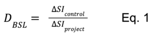
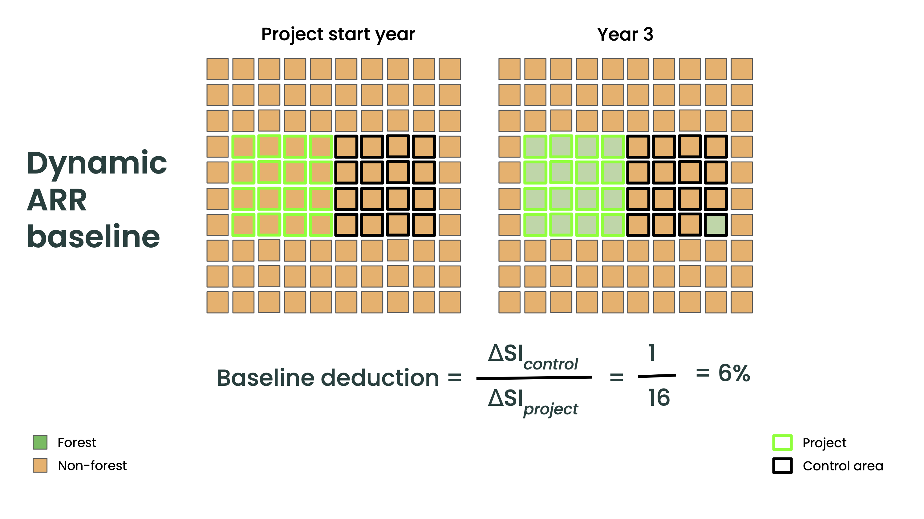
Fig. 4. Conceptual diagram of dynamic reforestation baseline. Left grid shows reforestation project (green borders) and control area (black borders) at project start. Right grid shows project and control area 3 years after project start. This simplified example shows reforestation of one grid cell in the control area and all 16 grid cells in the project, resulting in a 6% baseline deduction. This example also illustrates the difference between stocking indices (SI) sensitive to vegetation cover (e.g. satellite vegetation indices, such as NDVI) and SIs more sensitive to 3D forest structure (e.g., canopy height and carbon maps incorporating radar and lidar observations). Although satellite-derived vegetation indices are likely to detect the grid cells transitioning from non-forest to forest, SIs more sensitive to 3D forest structure are better able to track the ongoing carbon increase in these grid cells over time.

As specified in VM0047, ΔSI in the project and control are computed as the average annual project and control SI slopes since project start, using linear regression. To determine whether the difference in slopes (dΔ = ΔSIproject – ΔSIcontrol ) is statistically significant, VM0047 specifies a simple hypothesis test (H0: dΔ = 0, H1: dΔ ≠ 0), assuming independent standard errors on the slope coefficients (Eq. 2).ⁱ 

If ΔSIproject and ΔSIcontrol are statistically different, Eq. 1 is used to compute the baseline deduction. If not statistically different, the baseline deduction is 100%. We computed the project and control SI slopes and the corresponding baseline deductions at 3 and 4 years after the onset of reforestation at both test sites. 

Note that these rules for computing the baseline do not directly account for uncertainty in the SI.^j In future technical documentation, Pachama will describe in greater detail our methods for mapping canopy height (and ultimately carbon), including our methods for quantifying map uncertainty to produce confidence intervals on height (or carbon) change estimates for the project and control. As we discuss below, SI validation and uncertainty quantification will be essential for ensuring that baseline deductions are accurate and consistent across ARR projects.

Baseline uncertainty: pseudo-projects

As Pachama described in a previous research brief, baseline uncertainty can be quantified by computing baselines for pseudo-projects. In the case of reforestation, pseudo-projects are non-forest areas that are not enrolled in the carbon market. As neither pseudo-projects nor their control areas have a carbon project, their SI time series should match. Any discrepancies in the pseudo-project and control SI time series represent error in control area selection. We used the Mapbiomas land cover product to identify pseudo-projects: areas of constant pasture over 2000 – 2016, but unconstrained land use after 2016 (Fig. 1). We matched each pseudo-project to a control area using 2015 Pachama canopy height.

Non-zero baselines: plantations 

We used a commercial plantation within our study region to demonstrate performance of the dynamic baseline in cases of non-zero, albeit very large background carbon gain. Using a global map of planting years for tree plantations ¹⁸, we extracted an approximately 100-ha commercial plantation planted in 2017 (Fig. 1) and computed a dynamic baseline for this plantation. 

RESULTS

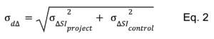
All stocking indices (SIs) exhibited statistically significant divergence between the test site and control SI in the initial years after the onset of reforestation (Fig. 5). However, within <5 years, NDVI (Landsat and Sentinel-2) reached its maximum value, whereas Pachama canopy height and ALOS-Palsar RNDVI did not saturate (Fig. 5). NDVI (Landsat and Sentinel-2) and RNDVI (ALOS-Palsar) also produced spurious baseline deductions as large as ~25% due to noise in the control area time series (Fig. 5a, b, c).

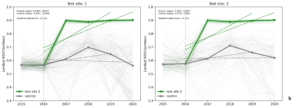
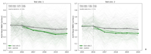
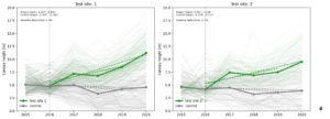
Fig. 5. Dynamic control area baseline for test sites. a) Landsat NDVI (30m), b) Sentinel-2 NDVI (10m), c) ALOS-Palsar RNDVI (25m), and d) Pachama canopy height (30m). The vertical line indicates the nominal year of reforestation (2016). Test sites are shown in green and their matching control areas in gray. Thin lines show the pixel-level SI time series and thick lines the mean test site and control are time series. Dashed lines indicate the SI change in test sites and their control areas 3 and 4 years after the nominal start of forest regrowth. Although Pachama pre-reforestation canopy height (2015 – 2016) is very likely overestimated, canopy height produced a zero baseline in line with what we expect for the region. If control area SI change is zero, project SI change is not required as long as it exceeds control area change (Fig. 4, Eq. 2). This is precisely why we recommend at least initially siting ARR projects in regions of minimal background reforestation. That way, one can avoid over-reliance on the accuracy of non-zero SI change until the market collectively evolves more rigorous, 3rd party map validation. In addition, Pachama is actively working to improve our height estimates over low vegetation areas and to validate our height change estimates against observed height change extracted from repeat airborne lidar.

Over constant land cover (forest, pasture, and crop) NDVI exhibits strong seasonal variability. In growing season months, mean NDVI over pasture and crops nearly reaches levels observed over forests (Fig. 6a). In contrast, Pachama canopy height remained nearly flat over constant pasture and crop cover (Fig. 6b). 

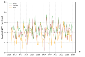
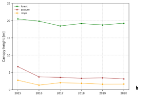
Fig. 6. Landsat NDVI (2013-2024) and Pachama canopy height (2015-2020) over constant forest, pasture, and crop cover. Panels show the median time series over each constant cover class (2000 – 2020). a) Monthly Landsat NDVI exhibits strong seasonal variability. In wetter months, with denser, greener vegetation, mean NDVI over pasture and crops can nearly reach the levels observed over forests. As an optical vegetation index, NDVI is effectively a proxy for chlorophyll absorption. It is most sensitive to leaf quantity and greenness as opposed to vertical forest structure. b) Canopy height derived from satellite observations using machine learning exhibits stability over constant cover and pronounced separation across cover types.

NDVI (Landsat and Sentinel-2) and RNDVI (ALOS-Palsar) exhibited weak correlation with observed height from airborne lidar, whereas Pachama canopy height estimates were strongly correlated with observed height (Fig. 7).

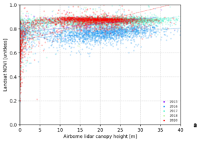
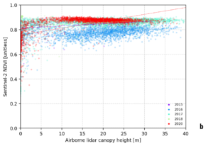
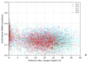
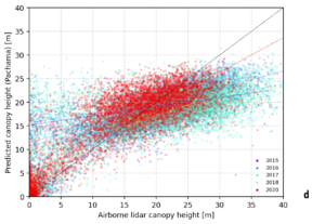
Fig. 7. Strength of correlation between stocking index (SI) and observed forest height from airborne lidar. a) Landsat NDVI (30m), b) Sentinel-2 NDVI (10m), c) ALOS-Palsar RNDVI (25m), and d) Pachama canopy height (30m). Each panel shows the pixel-level correlation between the SI and forest height measured from publicly available airborne lidar (Sustainable Landscapes and Reis and Jackson et al. 2022). Satellite-derived canopy height shows strong correlation with observed height from airborne lidar, whereas other candidate SIs exhibit significantly weaker correlation. Pachama is currently working to increase model skill at predicting canopy height >30m.

Our evaluation of the uncertainty of control area selection using pseudo-projects demonstrated tight annual match between mean canopy height in pseudo-projects and their controls. RMSE between project and control canopy height remained <1m one year after matching, increasing to ~2m 5 years after matching (Fig. 8).

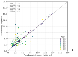
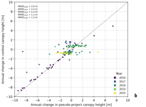
Fig. 8. Control area matching uncertainty. a) Annual forest height and b) annual change in forest height in pseudo-projects and their controls. Pseudo-projects are parcels that were continuously pasture (2000-2016) with no constraint on subsequent land use. Pixel-level kNN produces control areas that closely match each pseudo-project (pre-project matching year = 2015). As expected, the degree of similarity between pseudo-projects and their controls slightly declines in subsequent years.

Although registry rules should nearly always exclude commercial plantations from credit issuance for lack of additionality, the dynamic baseline computed for the test plantation produced the equivalent result (100% baseline deduction) without explicitly constraining the control area selection to other plantations. Due to the regular plantation cycle of growth and harvest, the test plantation’s canopy height time series (2015 – 2017) matched to other plantations with the same growth and harvest cycle. Consequently, height gain in the control area after 2017 mirrored height gain within the test plantation, resulting in a 100% baseline deduction (Fig. 9).

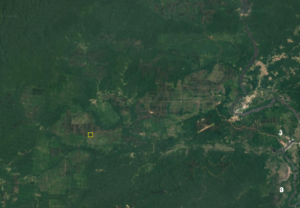
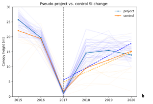
Fig. 9. Dynamic control area baseline for a commercial tree plantation. The expected baseline for our two natural regeneration test sites is near-zero, given the low background reforestation in the region. a) Here we use a sample 100-ha commercial tree plantation in Pará, Brazil planted in 2017 (yellow polygon) to demonstrate an example of a non-zero baseline. The control area was selected matching only on Pachama pre-project canopy height (2015-2017), using no ancillary map of commercial plantations in the region. b) Control area selection matches to other plantations, producing a baseline that follows the height gain trajectory of surrounding plantations (100% baseline deduction).

 

DISCUSSION

We computed a dynamic baseline for two test reforestation sites in Pará, Brazil across four candidate stocking indices (SIs). 

NDVI (Landsat and Sentinel-2) presented serious limitations as an SI (Fig. 5, Table 1), which is to be expected of vegetation indices derived from optical and near-infrared observations (e.g. NDVI, EVI, Red Edge Index, etc.) ¹⁹. These indices are primarily sensitive to chlorophyll, and are only weakly correlated with forest carbon (Fig. 7).^k NDVI exhibits large within-year variation associated with seasonal increases in vegetation greenness or density (Figs. 5, 6), even as tree height and diameter (i.e., carbon) remain roughly constant over these monthly time scales.

RNDVI (ALOS-Palsar) presented similar limitations, but, unlike NDVI, did not saturate in the early years after the onset of reforestation (Fig. 5, Table 1), as radar observations are expected to be more sensitive to vertical forest structure ²⁰.

Canopy height did not present these limitations. In addition, canopy height, unlike a vegetation index, is a quantity with clear physical meaning. This is a distinct advantage for transparency in crediting, as it makes sanity checks of ARR baselines much easier. For example, visiting an ARR project, one can roughly discern whether canopy height has increased by a few meters as opposed to whether a vegetation index has increased by some fractional amount.

Table 1. Stocking index (SI) performance for dynamic baseline

	Baseline deduction (%)  (Year 3)	Baseline deduction (%) (Year 4)	Saturation
Landsat NDVI	9, 0	0, 0	Yes
Sentinel-2 NDVI	25, 25	0, 0	Yes
ALOS – Palsar RNDVI	32, 27	28, 25	No
Pachama canopy height	0, 0	0, 0	No

 

This initial evaluation of candidate vegetation indices is not intended to be exhaustive, but rather illustrate the range of challenges to be expected if using minimally processed satellite data as a stocking index. 

Others certainly may achieve marginally better SI performance than we show here using different optical or radar vegetation indices or more thorough processing. Nonetheless, we expect such improvements to be fundamentally constrained by the specific sensor – optical and radar – limitations we’ve mentioned. 

For this reason, Pachama has concentrated on canopy height and carbon mapping using ground and airborne data for model training as opposed to pursuing more refined analysis of inherently limited vegetation indices.

Below we further discuss the performance of the candidate SIs, addressing four questions with key market implications we posed at the outset.

Year of first issuance 

Under current Verra requirements, a project cannot issue its first credits until SI gain within the project is statistically distinguishable from SI change within the control area. If an SI is weakly sensitive to early stages of reforestation, ARR projects may have to delay their first credit issuance.

All four candidate SIs exhibited statistically significant divergence between test sites and their control in < 5 years (Fig. 5).^l However, this is more an outcome of the methods specified in VM0047 (linear regression on pixel-level SI time series) than an actual indication of real SI (or carbon) divergence. 

Using pixel-level control area selection, even extremely small SI trends well within SI noise will be deemed statistically significant merely due to the number of pixels (i.e., large sample size). For example, a 100-ha project will have project and control sample sizes of 10,000 when using a 10m resolution SI and ~1,100 when using a 30m resolution SI.

In future technical documentation of Pachama’s canopy height mapping, we’ll discuss more robust methods for comparing project – control SI change (specifically canopy height) that account for SI uncertainty (i.e., how well canopy height predictions agree with observed canopy height).

Year of SI saturation

Computing an ARR dynamic baseline requires observing SI change in both the project and control area (Eq. 1). If an SI becomes insensitive to carbon gain, it is no longer a viable stocking index. 

Early saturation is particularly a risk for optical vegetation indices and two-dimensional quantities, such as canopy cover. These SIs can reach their maxima early in reforestation, because all pixels will contain relatively dense vegetation once the forest canopy closes, even though tree size and carbon content will continue to increase for decades. NDVI (Landsat and Sentinel-2) saturated within a year of the onset of reforestation (Fig. 5a,b). 

This is not the case for radar (ALOS-PALSAR Fig. 2c), which is more sensitive to vertical canopy structure. L-band radar (e.g., ALOS-PALSAR) generally does not saturate until carbon stocks reach ~50 Mg ha-1 ²¹, while the European Space Agency (ESA) BIOMASS instrument, to be launched in 2024, carries P-band radar, which is sensitive to much higher carbon stocks ²¹.

Similarly, Pachama canopy height derived from a suite of satellite observations, including ALOS-Palsar and Sentinel-1 radar, did not saturate at either test site (Fig. 3d). Pachama canopy height is not expected to saturate until reaching ~30m under Pachama’s current v0 mapping algorithm (Fig. S1), though we are improving our mapping algorithm to increase prediction accuracy for taller trees.

Accurate and consistent baselines

Accurate and consistent baselines are a necessity for building public confidence in carbon crediting. The noisier the SI, the larger the likely variation in baseline estimates for the same project.

Although Pachama canopy height produced the expected near-zero baseline, the optical and radar indices we evaluated produced baseline deductions ranging from 0 – 30% (Fig. 5, Table 1). Note that erroneously large baseline deductions (20-30%) mean a project would be under-credited, potentially harming its commercial viability.

Avoiding wide spread in estimated baseline deductions for the same test site will require 3rd-party SI validation against an independent, “ground-truth” database. Pachama has long advocated this paradigm shift to output-based validation of core crediting quantities. 

Satellite data enable crediting methods, such as dynamic baselines, that can better quantify project climate impact. But the complexity of this data and required preprocessing mean that current input-based crediting rules (e.g., Verra methodologies like VM00047) alone will not guarantee standardization in crediting outcomes.

Spurious increases in vegetation indices over control areas – unrelated to any actual carbon change – (Fig. 5) can have a range of proximate causes. In the case of optical indices, such as NDVI, these include atmospheric effects, sun-sensor geometry, and seasonal increases in vegetation “greenness” or transient increases following heavier rainfall (Fig. 6). Pachama canopy height, in contrast, was more stable over control areas (Fig. 5) and constant non-forest classes (Fig. 6), enabling more consistent, reproducible baselines. 

Minimum detectable baseline

ARR projects occur in areas with low existing carbon stocks, and consequently, will match to low carbon control areas. An SI is adequate only insofar as it is sufficiently sensitive to relatively small carbon changes from low initial carbon stocks. As mentioned previously, optical and radar vegetation indices were noisier than Pachama canopy height (Fig 5, Fig. 6, Table 1), and noisier SIs will be less able to detect smaller carbon changes. 

Conservative crediting requires an SI to detect small baselines. If an SI cannot reliably detect a 5% or 10% carbon gain, the baseline deduction in these cases will be zero, resulting in over-crediting. Pachama is beginning to address this question of minimum detectable baseline by validating our estimates of canopy height change against repeat airborne lidar observations. 

Finally, the minimum detectable baseline can have important implications for setting market rules around minimum allowable project size, as smaller reforestation projects will tend to have noisier SIs. 

NEXT STEPS

This Research Brief shows the potential for Verra’s newly released ARR methodology (VM00047) to ensure standardized, reproducible baselines for ARR projects. 

Consistent with a vast body of academic research, our results highlight the critical limitations of simpler SIs, particularly optical vegetation indices. 

First, these indices saturate too early in the course of reforestation to compute the dynamic baseline over a project’s lifetime. 

Second, due to the noisiness of simpler, “off the shelf” vegetation indices, they are unlikely to yield the accurate, reproducible baselines buyers and the public rightly expect. Baselines computed using these indices can be highly sensitive to methodological choices, such as compositing over the large seasonal variation in monthly observations to produce an annual SI time series.

We expect these findings to hold across additional ecoregions, as they result from fundamental limitations of different satellite sensors. We encourage other teams to publicly share similar SI testing to advance a collective understanding of suitable options. To facilitate such inter-comparison, you can download geojson boundary files with the test sites and pseudo-projects analyzed in this work (Fig. 1).

Together, our results indicate the market will likely need to adopt high-quality canopy height or carbon maps as the long-term SI solution unless other SI options are found to be suitable.

The urgent priority, therefore, is to accelerate the collective effort required to build the policy and compute infrastructure for 3rd-party map validation against independent, “ground-truth”. Ultimately, the core objective for this validation is to assess how well SI change tracks observed change in canopy height and carbon. Verra’s recently announced Forest Carbon Technical Working Group is a very promising step in this direction. 

Such an effort is foundational to giving buyers and the public the confidence that a project’s baseline would be the same regardless of the service provider producing the canopy height (or carbon) map.

FOOTNOTES

^a REDD: Reducing Emissions from Deforestation and Degradation.
^b ARR projects encompass afforestation, reforestation, and revegetation (ARR).
^c Though background reforestation rates in the absence of the carbon market can be quite small or near-zero⁶, forest regrowth on abandoned land can be significant in temperate and boreal regions^7–9 and tropical regions^10,11.
^d Note VM0047 uses the term dynamic performance benchmark to refer to a dynamic baseline.
^e We’ve also conducted initial ARR baseline tests in other ecoregions, namely the Brazilian Atlantic Forest and southeastern US, which confirm the findings we present here.
^f Pachama is undertaking some of this work to create cleaner forest age maps primarily to inform our regional estimates of expected carbon uptake over an ARR project’s lifetime.
^g Although other features, such as topography, distance to waterways, soil type, etc., could be used in control area selection, matching on pre-project SI time series alone (as minimally required by VM00047) shows tight project-control agreement when tested on pseudo-projects (RMSE < 1m, Fig. S2).
^h Equation A5 in VM00047 Appendix 1: Performance Method.
ⁱ Equation A6 in VM00047 Appendix 1: Performance Method.
^j The untested assumption implicit in VM0047 is that SI scales linearly with carbon, such that error is equivalent in the project and control area and canceled when computing the ratio of control-to-project SI change.
^k NDVI, for example, is a normalized ratio of chlorophyll absorption in the red band and leaf intercellular scattering in the near-infrared band ¹⁹.
^l Although all four candidate SIs exhibited sufficient divergence between test site and control, we have observed instances in which this is not the case, particularly where there may be existing vegetation on the site (i.e., the project is not bare ground prior to reforestation). In these cases, weak SI divergence between a project and control could delay first issuance.

REFERENCES

1. Forest Trends’ Ecosystem Marketplace. 2023. State of the Voluntary Carbon Markets 2023. Washington DC: Forest Trends Association.
2. Guizar‐Coutiño A, Jones JPG, Balmford A, Carmenta R, Coomes DA. A global evaluation of the effectiveness of voluntary REDD projects at reducing deforestation and degradation in the moist tropics. Conservation Biology. 2022. doi:10.1111/cobi.13970
3. West TAP, Börner J, Sills EO, Kontoleon A. Overstated carbon emission reductions from voluntary REDD+ projects in the Brazilian Amazon. Proc Natl Acad Sci U S A. 2020;117: 24188–24194.
4. West TAP, Wunder S, Sills EO, Börner J, Rifai SW, Neidermeier AN, et al. Action needed to make carbon offsets from tropical forest conservation work for climate change mitigation. arXiv; 2023. doi:10.48550/ARXIV.2301.03354
5. Mitchard ETA, Carstairs H, Cosenza R, Saatchi SS, Funk J, Quintano PN, et al. Serious errors impair an assessment of forest carbon projects: A rebuttal of West et al. (2023). arXiv [econ.GN]. 2023. Available: http://arxiv.org/abs/2312.06793
6. Crawford CL, Yin H, Radeloff VC, Wilcove DS. Rural land abandonment is too ephemeral to provide major benefits for biodiversity and climate. Sci Adv. 2022;8: eabm8999.
7. Lesiv M, Schepaschenko D, Moltchanova E, Bun R, Dürauer M, Prishchepov AV, et al. Spatial distribution of arable and abandoned land across former Soviet Union countries. Sci Data. 2018;5: 180056.
8. Schierhorn F, Müller D, Beringer T, Prishchepov AV, Kuemmerle T, Balmann A. Post-Soviet cropland abandonment and carbon sequestration in European Russia, Ukraine, and Belarus. Global Biogeochem Cycles. 2013;27: 1175–1185.
9. Yu Z, Lu C. Historical cropland expansion and abandonment in the continental U.S. during 1850 to 2016. Glob Ecol Biogeogr. 2018;27: 322–333.
10. Heinrich VHA, Dalagnol R, Cassol HLG, Rosan TM, de Almeida CT, Silva Junior CHL, et al. Large carbon sink potential of secondary forests in the Brazilian Amazon to mitigate climate change. Nat Commun. 2021;12: 1785.
11. Silva Junior CHL, Heinrich VHA, Freire ATG, Broggio IS, Rosan TM, Doblas J, et al. Benchmark maps of 33 years of secondary forest age for Brazil. Sci Data. 2020;7: 269.
12. David Shoch, Scott Settelmyer, John Furniss, Rebecca Dickson, Devon Ericksen, Igino Emmer. VM0047: Afforestation, Reforestation, and Revegetation. Verra; 2023 Sep. Available: https://verra.org/wp-content/uploads/2023/09/VM0047_ARR_v1.0-1.pdf
13. MapBiomas Project – Collection 71 of the Annual Land Use Land Cover Maps of Brazil, accessed on July 5, 2023 through the link: https://brasil.mapbiomas.org/en/colecoes-mapbiomas/.
14. Souza CM, Shimbo JZ, Rosa MR, Parente LL, Alencar AA, Rudorff BFT, et al. Reconstructing Three Decades of Land Use and Land Cover Changes in Brazilian Biomes with Landsat Archive and Earth Engine. Remote Sensing. 2020. p. 2735. doi:10.3390/rs12172735
15. Chen W, Yin H, Moriya K, Sakai T, Cao C. Retrieval and Comparison of Forest Leaf Area Index Based on Remote Sensing Data from AVNIR-2, Landsat-5 TM, MODIS, and PALSAR Sensors. ISPRS International Journal of Geo-Information. 2017;6: 179.
16. Dos-Santos MN, Keller MM. CMS: LiDAR Data for Forested Areas in Paragominas, Para, Brazil, 2012-2014. ORNL DAAC; 2016. doi:10.3334/ORNLDAAC/1302
17. Reis CR, Jackson TD, Gorgens EB, Dalagnol R, Jucker T, Nunes MH, et al. Forest disturbance and growth processes are reflected in the geographical distribution of large canopy gaps across the Brazilian Amazon. J Ecol. 2022;110: 2971–2983.
18. Du Z, Yu L, Yang J, Xu Y, Chen B, Peng S, et al. A global map of planting years of plantations. Sci Data. 2022;9: 141.
19. Huang S, Tang L, Hupy JP, Wang Y, Shao G. A commentary review on the use of normalized difference vegetation index (NDVI) in the era of popular remote sensing. Res J For. 2020;32: 1–6.
20. Pardini M, Armston J, Qi W, Lee SK, Tello M, Cazcarra Bes V, et al. Early Lessons on Combining Lidar and Multi-baseline SAR Measurements for Forest Structure Characterization. Surv Geophys. 2019;40: 803–837.
21. Woodhouse IH, Mitchard ETA, Brolly M, Maniatis D, Ryan CM. Radar backscatter is not a “direct measure” of forest biomass. Nat Clim Chang. 2012;2: 556–557.